Optimizing data throughput for Postgres snapshots with batch size auto-tuning
Why static batch size configuration breaks down in real world networks and how automatic batch size tuning improves snapshot throughput.
By:
Esther Minano SanzPublished:
Reading time:
7 min readFor many production setups, taking a database snapshot involves transferring significant amounts of data over the network. The standard way to do this efficiently is to process data in batches. Batching reduces per-request overhead and helps maximize throughput, but it also introduces an important tuning problem: choosing the right batch size.
A batch size that works well in a low latency environment can become a bottleneck when snapshots run across regions or under less predictable network conditions. Static batch size configuration assumes stable networks, which rarely reflects reality.
In this blog post we describe how we used automatic batch size tuning to optimize data throughput for Postgres snapshots, the constraints we worked under and how we validated that the approach actually improves performance in production-like environments for our open source pgstream tool.
💡pgstream is an open source CDC tool built around PostgreSQL logical replication. It supports DDL changes, initial snapshots, continuous replication and column level transformations for data anonymization. Learn more here.
Why batch sizing is tricky
At Xata, we use pgstream to migrate customer databases into our platform. During the initial snapshot, the amount of data transferred over the network and written to the target database can slow progress significantly if the right batch size isn’t used. While pgstream has no control over external conditions, choosing the right batch configuration can make a meaningful difference.
However, determining the optimal setting is difficult, as it often varies across environments and customers. Manual tuning does not scale, and default values are inevitably wrong for some setups. Network conditions are also constantly changing (congestion, noisy neighbors)- what is optimal one day might not be the next!
What we wanted from a solution
At a high level, we wanted a way to automatically find a good batch size by measuring throughput in bytes per second across different configurations and picking the best one. Once a good value is identified, it can be used for the rest of the snapshot.
Rather than trying to model the system or predict performance, the idea was to keep things simple: observe how the system behaves under real conditions and move toward configurations that perform better.
With that in mind, we set a few clear constraints before thinking about specific algorithms:
- It should adapt automatically to different environments
- It should converge quickly and predictably
- It should be simple enough to reason about and maintain
- It should behave well on unstable networks
- It should fail safely when tuning is not possible
The auto-tuning implementation
With those constraints in place, the next question was how to actually build this in a way that stayed simple and predictable. We did not want a complex model or a tuning process that was hard to debug or could deviate from reality as code or usage patterns changed.
Instead, we chose a directional binary search. It gave us a straightforward way to explore the batch size space, react to what we observed and converge quickly without adding too much complexity.
Given a range of batch sizes to evaluate, the implementation:
- Measures throughput at the midpoint of the range
- Checks whether increasing or decreasing the batch size improves throughput
- Moves in the direction that looks better
- Converges once it starts oscillating between two adjacent values
This algorithm works best when throughput follows a single peak or a mostly flat curve, which is a common pattern in network-bound workloads. As batch size increases, throughput typically improves up to the point where latency, buffering, or congestion start to dominate, after which gains level off or drop. In these conditions, the algorithm can reliably move toward higher throughput and converge on a good batch size.
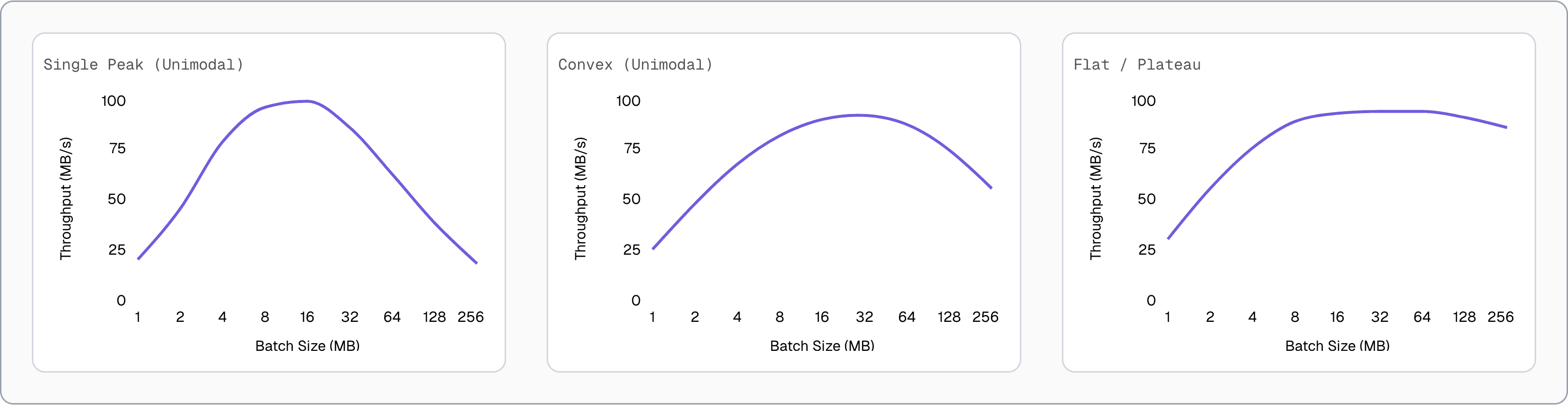
⚠️ With highly variable network latency (lots of “jitter”), throughput can swing from one batch to the next regardless of batch size. In that case, there is no single “right” batch size to converge on.
Practical constraints and safeguards
In the real world, things are rarely as clean as the algorithm assumes. Network hiccups, timeouts and noisy measurements all need to be accounted for. To make auto-tuning reliable in practice we added a few safeguards.
Making measurements meaningful
Throughput measurements need to be meaningful. A single data point is not enough, since it could be influenced by temporary network conditions. To avoid this, the algorithm enforces a minimum number of samples before comparing configurations. Once enough samples are collected, it uses the average throughput.
Batch processing also depends on more than just batch size. Timeouts are commonly used to ensure progress does not stall when traffic is slow. This means batches may never reach their configured size. That typically happens in two cases:
- The dataset is too small
- Data arrives too slowly and the timeout fires before the batch fills, meaning the system is already operating at capacity
In both cases, no further auto-tuning is necessary.
Dealing with instability
Early measurements are often noisy. This usually happens while the operating system’s TCP auto-tuning adjusts to the network conditions. Using those measurements can push the algorithm in the wrong direction.
To handle this, we track the Coefficient of Variation (CoV), also known as relative standard deviation. When the variance is low, we know we have a consistent measurement. We compute it over the last three samples so only recent behavior is considered. If the CoV exceeds a defined threshold, the algorithm keeps collecting samples until things stabilize.
If the network remains unstable and none of the measurements fall below the CoV threshold, auto-tuning stops and the default configuration is used instead.
💡 This algorithm prioritizes simplicity, maintainability and practical effectiveness across real world scenarios - more optimal algorithms may exist!
If you want to dig into the implementation details, you can take a look at the PR where the algorithm was introduced.
Validating behavior with property tests
Even with safeguards in place, we needed confidence that the implementation behaved correctly under all conditions. While the algorithm itself is conceptually simple, implementing it correctly while handling all edge cases can be difficult. Validation is crucial in this kind of situation, and unit testing can only get you so far. Cue one of the most underused validation tools…property testing! 🧪
Property tests let you define rules or invariants that your code must satisfy, instead of providing a series of input/outputs. Then a testing engine (we used rapid) checks the properties you define hold for a large number of automatically generated test cases.
The hardest part is identifying the right invariants. In our case, they fell into a few groups:
- Convergence: the algorithm converges within bounded iterations
- Correctness: it finds an optimal or near-optimal batch size
- Safety: throughput never regresses and the search space always narrows
- Stability: unstable measurements are retried or rejected
- Failure handling: tuning stops when stability cannot be achieved
These properties give us confidence that the algorithm behaves predictably and safely as it evolves. You can find the full set of property tests here.
Benchmarks
Now, property tests are great for validating the correctness of the algorithm implementation, but we also needed benchmarks that would show it actually improved performance!
Since the problem is network related, benchmarks needed to be representative of real world conditions. We focused on two common production scenarios:
- Cross-region source and target:
pgstreamruns in an EC2 instance, with both the source and target databases located in different regions. This setup introduces network latency on both the read and write paths. - Local source, remote target:
pgstreamruns in the same region as the source database, but the target database is in a different region. In this case, reads are fast and local, while writes are constrained by cross-region latency.
To simulate network conditions, we used the network emulator module (netem) via the Linux traffic control utility (tc) and tested:
- Normal: Ideal network with low latency and high bandwidth
- Slow: Simulated latency of 200 ms ±10 ms jitter
- Very Slow: Simulated latency of 500 ms ±20 ms jitter
Benchmarks were run in pairs (auto-tuned vs manual batch size) using a 2 GB table (cast_info) from the IMDB database. The manual runs used the current default settings of 80 MB batch size and 30s timeout. Full benchmark setup details are available here.
Results and takeaways
In ideal network conditions, batch size had minimal impact on performance. Auto-tune selected a significantly smaller batch size (24.7 MB vs 80 MB) with near-identical performance through 9 iterations of binary search, demonstrating that batch size doesn't make a major difference when network speed is not the limiting factor.
For slow network conditions, the default 80 MB configuration was severely oversized, causing 3.4x throughput loss consistently across 6 runs. Auto-tune correctly identified ~50 MB as optimal through efficient binary search, saving 23 minutes per snapshot (32 min → 9 min) 🚀. All runs followed the same convergence path, demonstrating the algorithm's deterministic behavior and reliability.
In very slow networks, the default 80 MB configuration caused catastrophic performance degradation. The oversized batches led to network buffer saturation, increased timeouts and memory pressure, with the system throughput dropping to 422 kB/s by the end. Auto-tune's 49.7 MB selection completed in 23 minutes vs 1h 22 minutes - a 3.5x speedup! 🏎️
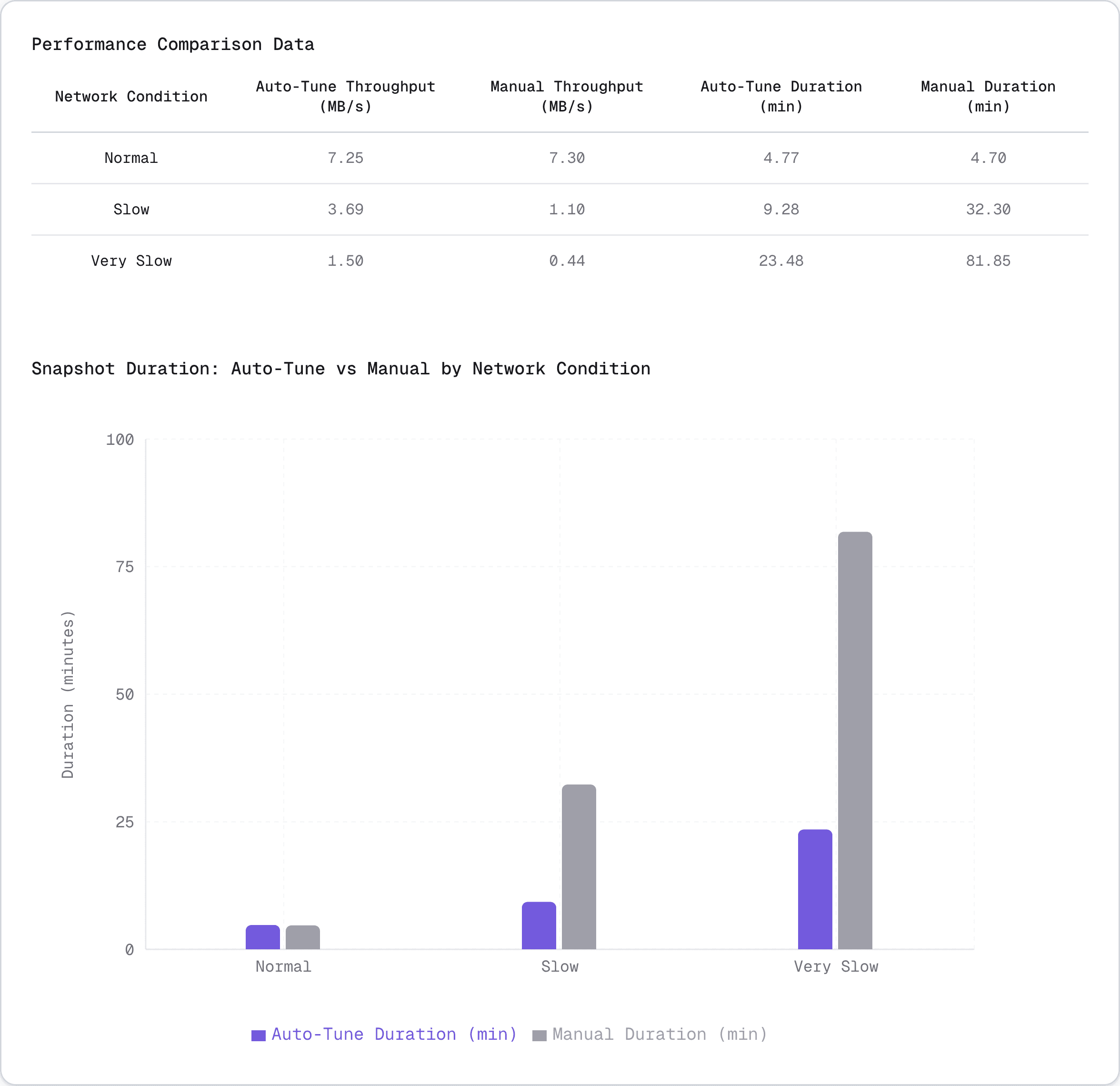
⚡ Performance insights
- Throughput improvement: Up to 2.5× higher throughput compared to manual configuration
- Duration reduction: Average duration reduced by 45%
Auto-tuning delivered significant performance improvements in network-constrained environments while maintaining equivalent performance in ideal conditions. The algorithm reliably found batch sizes that avoided both undersized and oversized configurations.
Conclusion
The approach outlined in this blog post is intentionally simple but effective. By combining directional search, basic statistical stability checks, and strong validation through property testing, it is possible to build adaptive systems that behave correctly and predictably without excessive complexity. This pattern is broadly applicable to batch processors, data pipelines, and ingestion systems where workload characteristics are not known in advance.
It allowed us to make pgstream more adaptive to real production conditions without increasing operational complexity for users. For large tables, long running snapshots and latency sensitive networks, the gains far outweigh the initial tuning cost.
If you run pgstream in environments with unusual network characteristics or edge cases we have not covered, we would love to hear about it. Please share your experience through issues, or contribute improvements via pull requests.
To opt-in to this pgstream feature, you just need to enable it in your target Postgres configuration:
Ready to try it on Xata? Get access here and start migrating your database to our platform.
Give every agentic workload its own Postgres branch
Create instant database clones with production-like data for every agent, workflow, and CI/CD pipeline.
Related Posts
Behind the scenes: Speeding up pgstream snapshots for PostgreSQL
How targeted improvements helped us speed up bulk data loads and complex schemas.
pgstream v0.9.0: Better schema replication, snapshots and cloud support
Bringing connection retries, anonymizer features, memory improvements and solid community input.
pgstream v0.8.1: hstore transformer, roles snapshotting, CLI improvements and more
Learn how pgstream v0.8.1 transforms hstore data and improves snapshot experience with roles snapshotting and excluded tables option
pgstream v0.7.1: JSON transformers, progress tracking and wildcard support for snapshots
Learn how pgstream v0.7.1 transforms JSON data, improves snapshot experience with progress tracking and wildcard support.
pgstream v0.6.0: Template transformers, observability, and performance improvements
Learn how pgstream v0.6 simplifies complex data transformations with custom templates, enhances observability and improves snapshot performance.
pgstream v0.5.0: New transformers, YAML configuration, CLI refactoring & table filtering
Improved user experience with new transformers, YAML configuration, CLI refactoring and table filtering.
pgstream v0.4.0: Postgres-to-Postgres replication, snapshots & transformations
Learn how the latest features in pgstream refine Postgres replication with near real-time data capture, consistent snapshots, and column-level transformations.
Introducing pgstream: Postgres replication with DDL changes
Today we’re excited to expand our open source Postgres platform with pgstream, a CDC command line tool and library for PostgreSQL with replication support for DDL changes to any provided output.
Postgres Cafe: Solving schema replication gaps with pgstream
In this episode of Postgres Café, we discuss pgstream, an open-source tool for capturing and replicating schema and data changes in PostgreSQL. Learn how it solves schema replication challenges and enhances data pipelines.
Postgres webhooks with pgstream
Trigger HTTP webhooks on every INSERT, UPDATE, or DELETE in PostgreSQL. Open-source CDC setup with pgstream, no polling required.